Saved notebook output; this documentation build does not execute cells. Download the notebook.

A four-cell sea-surface temperature sample

Fetch a tiny NOAA CoastWatch subset, inspect its units, and visualize the four grid centers. This uses usdata v0.6 or newer and the optional pandas reader.

Saved outputs are a recorded run. The execution and source retrieval times below identify the snapshot. NOAA may revise data; a future run can differ. Run Restart Kernel and Run All Cells to reproduce the workflow, or change the query cell to explore another small region and timestamp.

See examples setup for the optional environment and execution commands.

from datetime import UTC, datetime

import pandas as pd
from IPython.display import Markdown, display

import usdata
from usdata import build_query, get
from usdata.fetch import fetch

pd.set_option("display.max_rows", 8)
pd.set_option("display.max_columns", 8)
print(f"Executed (UTC): {datetime.now(UTC).isoformat(timespec='seconds')}")
print(f"usdata {usdata.__version__}; pandas {pd.__version__}")

Executed (UTC): 2026-09-09T00:11:44+00:00
usdata 0.7.0; pandas 3.0.5

1. Select the input

Bounds are (west, south, east, north). These coordinates select four ocean grid centers at one analysis time. Keep exploratory subsets small; date-only bounds mean midnight, whereas this dataset's analyses are at noon UTC.

dataset = get("noaa:coastwatch-sst")
query = build_query(
    bbox=(-80.08, 30.02, -80.02, 30.08),
    start="2024-05-06T12:00Z",
    end="2024-05-06T12:00Z",
    variables=["analysed_sst"],
)
items = fetch(dataset, query)
(item,) = items
frame = item.open(parse_dates=["time"])
display(frame.round({"latitude": 3, "longitude": 3, "analysed_sst": 3}))

	time	latitude	longitude	analysed_sst
0	2024-05-06 12:00:00+00:00	30.025	-80.075	26.85
1	2024-05-06 12:00:00+00:00	30.025	-80.025	26.99
2	2024-05-06 12:00:00+00:00	30.075	-80.075	26.78
3	2024-05-06 12:00:00+00:00	30.075	-80.025	26.95

2. Inspect units and provenance

ERDDAP's second CSV record contains units. The reader moves it into metadata instead of treating it as an observation. Coordinates, measurements, and units stay in their original scientific conventions; no unit conversion occurs.

units = frame.attrs["units"]
display(pd.Series(units, name="source units").to_frame())

	source units
time	UTC
latitude	degrees_north
longitude	degrees_east
analysed_sst	degree_C

for item in items:
    print(f"{item.asset.dataset_id}")
    print(f"Retrieved (UTC): {item.provenance.retrieved_at.isoformat()}")
    print(f"Bytes: {item.provenance.size}; cache hit: {item.from_cache}")
    print(f"Checksum: {item.provenance.checksum}")
    display(Markdown(f"[Source request](<{item.provenance.source_url}>)"))

noaa:coastwatch-sst
Retrieved (UTC): 2026-09-09T00:11:44.923930+00:00
Bytes: 261; cache hit: False
Checksum: sha256:161d5cd3383fb2a6601d298aedd07f16966a47742881204115a1361c5b2a9a2e

Source request

3. Summarize and plot

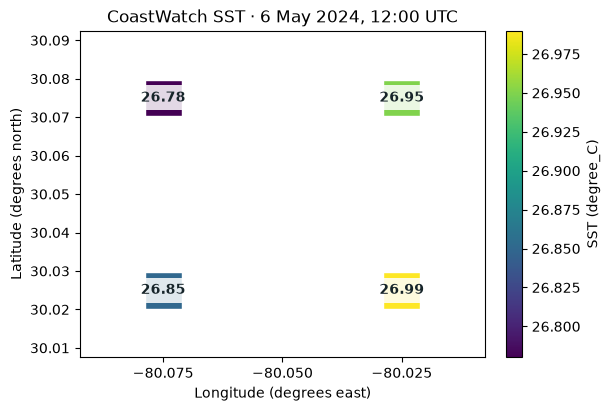
This is an unweighted mean of four nearby grid centers, not a regional or climate statistic. The axes show grid coordinates, not a projected map. The color scale applies only to this small sample.

print(f"{len(frame)} cells; mean SST: {frame['analysed_sst'].mean():.2f} {units['analysed_sst']}")

4 cells; mean SST: 26.89 degree_C

%matplotlib inline
import matplotlib.pyplot as plt
from matplotlib.ticker import MaxNLocator

fig, ax = plt.subplots(figsize=(6, 4), layout="constrained")
points = ax.scatter(
    frame["longitude"],
    frame["latitude"],
    c=frame["analysed_sst"],
    s=700,
    marker="s",
    cmap="viridis",
    edgecolors="white",
)
for row in frame.itertuples():
    ax.annotate(
        f"{row.analysed_sst:.2f}",
        (row.longitude, row.latitude),
        ha="center",
        va="center",
        color="#17252a",
        weight="bold",
        bbox={"facecolor": "white", "alpha": 0.85, "edgecolor": "none"},
    )
ax.set(
    xlabel="Longitude (degrees east)",
    ylabel="Latitude (degrees north)",
    title="CoastWatch SST · 6 May 2024, 12:00 UTC",
)
ax.ticklabel_format(useOffset=False)
ax.xaxis.set_major_locator(MaxNLocator(nbins=4))
ax.margins(0.35)
fig.colorbar(points, ax=ax, label=f"SST ({units['analysed_sst']})")
plt.show()

png

4. Reuse the cached input

Fetching the same query again validates and reuses the cached file. Editing frame leaves the raw CSV and provenance untouched. For a persistent set of pinned inputs, use a manifest as in the monthly climate notebook.

(cached,) = fetch(dataset, query)
print(f"Second fetch used cache: {cached.from_cache}")
print(f"Same checksum: {cached.provenance.checksum == item.provenance.checksum}")

Second fetch used cache: True
Same checksum: True